Shared metrics (raw output)
This page is meant to share reproducible metrics for each stage of the full chain. Feel free to open it in Binder to customize the visualization.
Warning
None of these metrics are convolved with the analysis tools.
Note
Technical details
Config location: config/chain/metrics.cfg
Sample was generated with MPV/MPR generator using icaruscode v09_49_00.
import numpy as np
import pandas as pd

import matplotlib
from matplotlib import pyplot as plt
import seaborn
seaborn.set(rc={
    'figure.figsize':(15, 10),
})
seaborn.set_context('talk') # or paper
import os
METRICS_FOLDER = '/sdf/group/neutrino/ldomine/chain/me/mpvmpr_062022/log_metrics3/'
UResNet
Confusion matrix
def plot_confusion_matrix(cm,
                          normalize=False,
                          title=None,
                          cmap=plt.cm.Blues,
                         xlabel='Predicted label',
                         ylabel='True label',
                         xticklabels=['Shower', 'Track', 'Michel', 'Delta', 'LowE'],
                         yticklabels=['Shower', 'Track', 'Michel', 'Delta', 'LowE'],
                         show_colorbar=True):
    """
    This function prints and plots the confusion matrix.
    Normalization can be applied by setting `normalize=True`.
    """
    fig, ax = plt.subplots()
    #print(cm.shape)
    im = ax.imshow(cm, interpolation='nearest', cmap=cmap)
    if show_colorbar:
        ax.figure.colorbar(im, ax=ax)
    #labels = ['HIP', 'MIP', 'Shower', 'Delta', 'Michel']
    labels = yticklabels
    # We want to show all ticks...
    ax.set(xticks=np.arange(cm.shape[1]),
           yticks=np.arange(cm.shape[0]),
           # ... and label them with the respective list entries
           xticklabels=xticklabels, yticklabels=labels,
           title=title,
           ylabel=ylabel,
           xlabel=xlabel,
           ylim=(-0.5, cm.shape[0]-0.5))

    # Rotate the tick labels and set their alignment.
    plt.setp(ax.get_xticklabels(), rotation=45, ha="right",
             rotation_mode="anchor")

    # Loop over data dimensions and create text annotations.
    fmt = '.2f'
    thresh = cm.max() / 2.
    for i in range(cm.shape[0]):
        for j in range(cm.shape[1]):
            ax.text(j, i, format(cm[i, j], fmt),
                    ha="center", va="center",
                    color="white" if cm[i, j] > thresh else "black")
    fig.tight_layout()
    return ax
from numpy.linalg import norm
range = __builtins__.range

def confusion_matrix(metrics, num_classes):
    x = np.zeros((num_classes+1, num_classes+1))
    for c in range(num_classes):
        for c2 in range(num_classes):
            x[c][c2] = np.nansum(metrics['confusion_%d_%d' % (c, c2)])
        x[c][-1] = np.nansum(metrics['num_true_pix_class%d' % c]-metrics['num_true_deghost_pix_class%d' % c])
        x[num_classes][c] = np.nansum(metrics['ghost2nonghost_class%d' % c])
    x[num_classes, num_classes] = np.nansum((metrics['ghost2ghost'])*metrics['num_ghost_points'])
    return x / x.sum(axis=1, keepdims=True)

def confusion_matrix2(metrics, num_classes):
    x = np.zeros((num_classes, num_classes))
    for c in range(num_classes):
        for c2 in range(num_classes):
            x[c][c2] = np.nansum(metrics['confusion_%d_%d' % (c, c2)])
    return x / x.sum(axis=1, keepdims=True)
deghosting = pd.read_csv(os.path.join(METRICS_FOLDER, 'deghosting_metrics.csv'))
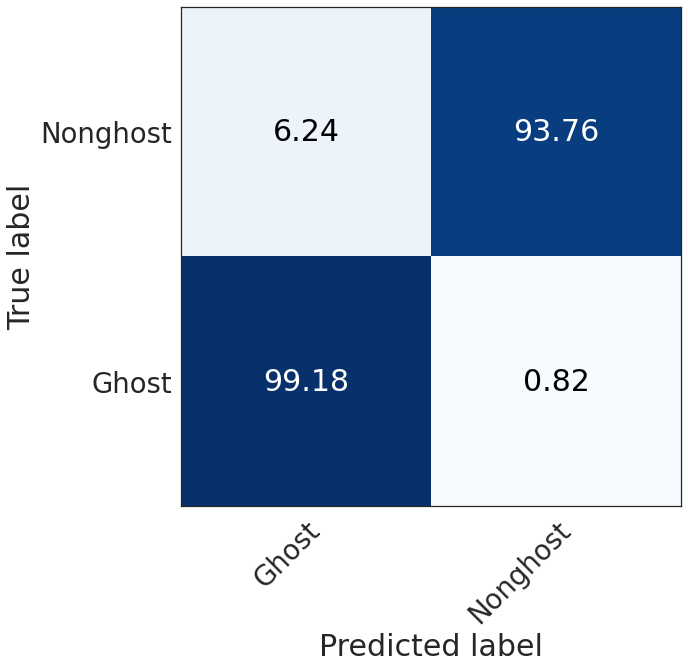
Ghost vs nonghost confusion matrix
cm = np.empty((2, 2))

cm[0, 0] = (deghosting['ghost2ghost']*deghosting['num_ghost_points']).sum()
cm[0, 1] = (deghosting['num_ghost_points'] * (1 - deghosting['ghost2ghost'])).sum()
cm[1, 1] = (deghosting['nonghost2nonghost'] * deghosting['num_nonghost_points']).sum()
cm[1, 0] = (deghosting['num_nonghost_points']* (1 -deghosting['nonghost2nonghost'] )).sum()

cm[0, :] /= cm[0, :].sum()
cm[1, :] /= cm[1, :].sum()

seaborn.set(style="white", font_scale=2.5)
plot_confusion_matrix(np.array(cm*100),
                      show_colorbar=False,
                     xticklabels=['Ghost', 'Nonghost'],
                     yticklabels=['Ghost', 'Nonghost'])

seaborn.set(rc={
    'figure.figsize':(15, 10),
})
seaborn.set_context('talk')
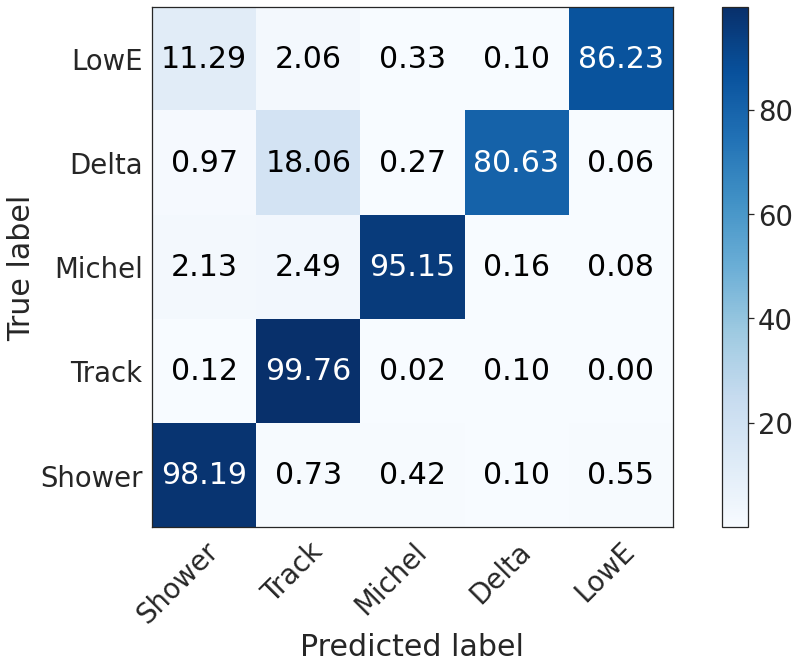
Semantic confusion matrix, nonghost only
We restrict the voxels to the true nonghost voxels correctly predicted as nonghost.
seaborn.set(style="white", font_scale=2.5)
plot_confusion_matrix(np.array(confusion_matrix2(deghosting, 5)*100))

seaborn.set(rc={
    'figure.figsize':(15, 10),
})
seaborn.set_context('talk')
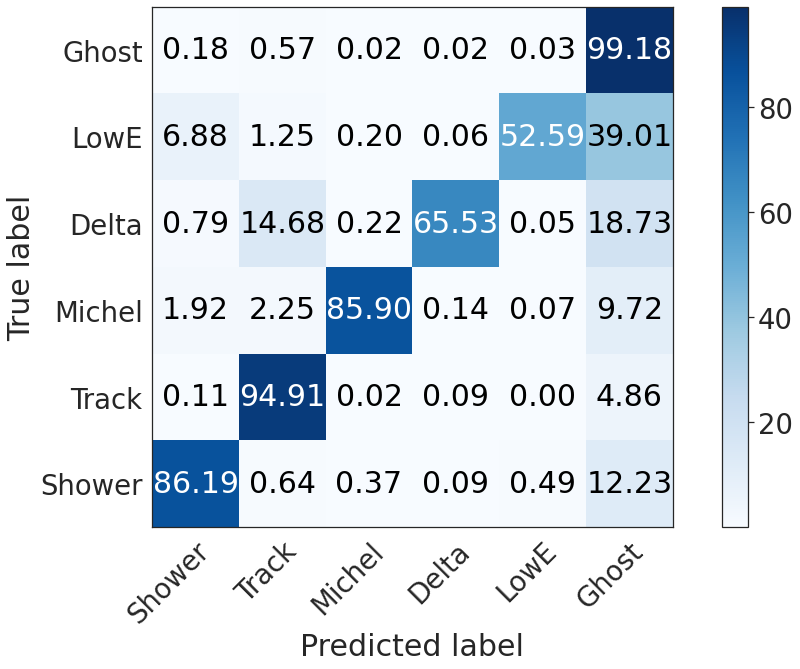
Global semantic confusion matrix (including ghosts)
seaborn.set(style="white", font_scale=2.5)
plot_confusion_matrix(np.array(confusion_matrix(deghosting, 5)*100),
                     xticklabels = ['Shower', 'Track', 'Michel', 'Delta', 'LowE', 'Ghost'],
                     yticklabels = ['Shower', 'Track', 'Michel', 'Delta', 'LowE', 'Ghost'])

seaborn.set(rc={
    'figure.figsize':(15, 10),
})
seaborn.set_context('talk')
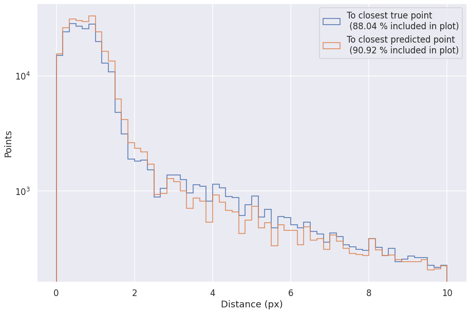
PPN
logs_gt = pd.read_csv(os.path.join(METRICS_FOLDER, "ppn-metrics-gt.csv"))
logs_pred = pd.read_csv(os.path.join(METRICS_FOLDER, "ppn-metrics-pred.csv"))
no_delta_pred = logs_pred['score_type_3'] < 0.5

#print("After removing delta points, keeping:", np.count_nonzero(no_delta_pred)/no_delta_pred.shape[0])

r = [0, 10]
bins = 60 #25
f= plt.figure()

fraction1 = np.count_nonzero(logs_pred[no_delta_pred]['min_distance']<r[1])/len(logs_pred[no_delta_pred])
plt.hist(logs_pred[no_delta_pred]['min_distance'], range=r, bins=bins, histtype='step', label='To closest true point \n (%.2f %% included in plot)' % (fraction1*100))

#print("Fraction of predicted points included in plot = ", fraction1)
print("Median of pred. points within 3px of true point = ", np.median(logs_pred[no_delta_pred]['min_distance'][logs_pred[no_delta_pred]['min_distance']<3]))
print("Median of pred. points within 5px of true point = ", np.median(logs_pred[no_delta_pred]['min_distance'][logs_pred[no_delta_pred]['min_distance']<5]))

no_delta_gt = logs_gt['Class'] != 3
fraction2 =  np.count_nonzero(logs_gt[no_delta_gt]['min_distance']<r[1])/len(logs_gt[no_delta_gt])
plt.hist(logs_gt[no_delta_gt]['min_distance'], range=r, bins=bins, histtype='step', label='To closest predicted point \n (%.2f %% included in plot)' % (fraction2*100))

plt.legend()
plt.yscale('log')
plt.xlabel('Distance (px)')
plt.ylabel('Points')
#print("Fraction of true points included in plot = ", fraction2)
Median of pred. points within 3px of true point =  0.73424
Median of pred. points within 5px of true point =  0.77339
Text(0, 0.5, 'Points')
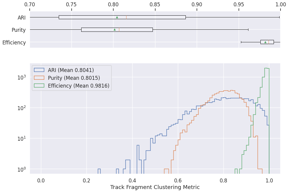
GraphSpice (CNN clustering)
graph_spice = pd.read_csv(os.path.join(METRICS_FOLDER, "graph-spice-metrics.csv"))

nonzero_ari = graph_spice['ARI'] > 0
# print(np.count_nonzero(nonzero_ari)/len(graph_spice))
fig, axs = plt.subplots(2,1, gridspec_kw={'height_ratios': [1, 3]})

axs[0].boxplot([
    graph_spice['efficiency'][nonzero_ari],
    graph_spice['purity'][nonzero_ari],
    graph_spice['ARI'][nonzero_ari]
    ], vert=False, showmeans=True,showfliers=False)
axs[0].set_yticklabels(['Efficiency', 'Purity', 'ARI'])
axs[0].set_xlim(0.7, 1.)
axs[0].xaxis.tick_top()

axs[1].hist(graph_spice['ARI'][nonzero_ari], range=[0, 1], bins=100, label='ARI (Mean %.4f)' % graph_spice['ARI'][nonzero_ari].mean(), histtype='step')
axs[1].hist(graph_spice['purity'][nonzero_ari], range=[0, 1], bins=100, label='Purity (Mean %.4f)' % graph_spice['purity'][nonzero_ari].mean(), histtype='step')
axs[1].hist(graph_spice['efficiency'][nonzero_ari], range=[0, 1], bins=100, label='Efficiency (Mean %.4f)' % graph_spice['efficiency'][nonzero_ari].mean(), histtype='step')
plt.legend(loc='upper left')
plt.yscale('log')
plt.xlabel('Track Fragment Clustering Metric')
Text(0.5, 0, 'Track Fragment Clustering Metric')
Grappa
Shower clustering
logs = pd.read_csv(os.path.join(METRICS_FOLDER, "cluster-gnn-metrics-shower.csv"))

fig, axs = plt.subplots(2,1, gridspec_kw={'height_ratios': [1, 3]})

axs[0].boxplot([
    logs['eff'][logs['ari']>0],
    logs['pur'][logs['ari']>0],
    logs['ari'][logs['ari']>0]
    ], vert=False, showmeans=True,showfliers=False)
axs[0].set_yticklabels(['Efficiency', 'Purity', 'ARI', ])
axs[0].set_xlim(0.96, 1.)
axs[0].xaxis.tick_top()

axs[1].hist(logs['ari'][logs['ari']>0], label="ARI (Mean: %.4f)" % logs['ari'][logs['ari']>0].mean(), histtype='step', range=[0, 1], bins=100)
axs[1].hist(logs['pur'][logs['ari']>0], label="Purity (Mean: %.4f)" % logs['pur'][logs['ari']>0].mean(), histtype='step', range=[0, 1], bins=100)
axs[1].hist(logs['eff'][logs['ari']>0], label="Efficiency (Mean: %.4f)" % logs['eff'][logs['ari']>0].mean(), histtype='step', range=[0, 1], bins=100)
plt.legend(loc='upper left')
plt.yscale('log')
plt.xlabel('Shower Clustering Metric')
Text(0.5, 0, 'Shower Clustering Metric')
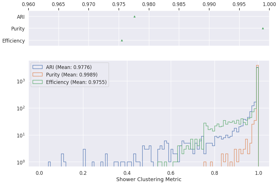
print("Accuracy of primary shower fragment identification: %.1f%%" % (logs['primary_accuracy'].mean()*100))
Accuracy of primary shower fragment identification: 68.6%
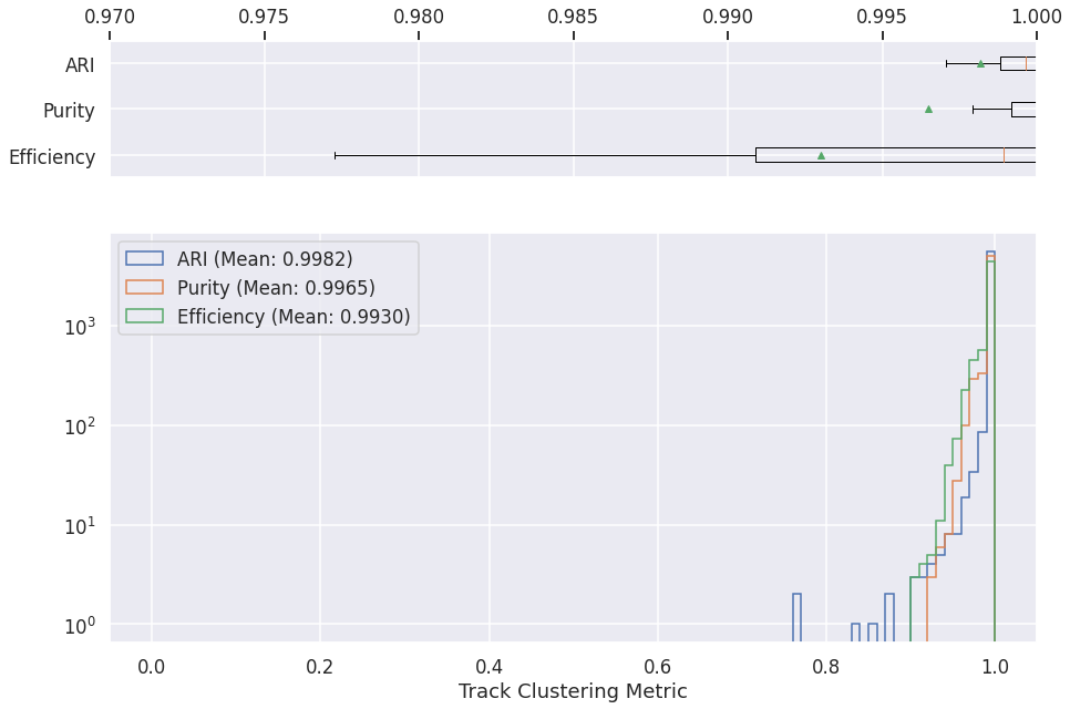
Track clustering
logs = pd.read_csv(os.path.join(METRICS_FOLDER, "cluster-gnn-metrics-track.csv"))

fig, axs = plt.subplots(2,1, gridspec_kw={'height_ratios': [1, 3]})

axs[0].boxplot([
    logs['eff'][logs['ari']>0],
    logs['pur'][logs['ari']>0],
    logs['ari'][logs['ari']>0]
    ], vert=False, showmeans=True,showfliers=False)
axs[0].set_yticklabels(['Efficiency', 'Purity', 'ARI', ])
axs[0].set_xlim(0.97, 1.)
axs[0].xaxis.tick_top()

axs[1].hist(logs['ari'][logs['ari']>0], label="ARI (Mean: %.4f)" % logs['ari'][logs['ari']>0].mean(), histtype='step', range=[0, 1], bins=100)
axs[1].hist(logs['pur'][logs['ari']>0], label="Purity (Mean: %.4f)" % logs['pur'][logs['ari']>0].mean(), histtype='step', range=[0, 1], bins=100)
axs[1].hist(logs['eff'][logs['ari']>0], label="Efficiency (Mean: %.4f)" % logs['eff'][logs['ari']>0].mean(), histtype='step', range=[0, 1], bins=100)
plt.legend(loc='upper left')
plt.yscale('log')
plt.xlabel('Track Clustering Metric')
Text(0.5, 0, 'Track Clustering Metric')
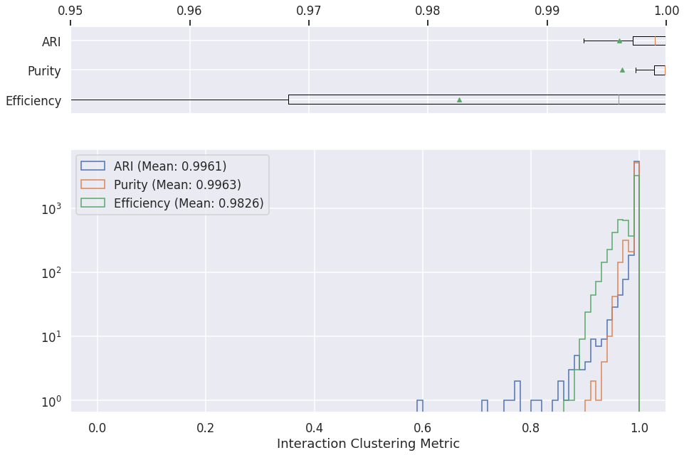
Interaction clustering
logs = pd.read_csv(os.path.join(METRICS_FOLDER, "cluster-gnn-metrics-inter.csv"))

fig, axs = plt.subplots(2,1, gridspec_kw={'height_ratios': [1, 3]})

axs[0].boxplot([
    logs['eff'][logs['ari']>0],
    logs['pur'][logs['ari']>0],
    logs['ari'][logs['ari']>0]
    ], vert=False, showmeans=True,showfliers=False)
axs[0].set_yticklabels(['Efficiency', 'Purity', 'ARI', ])
axs[0].set_xlim(0.95, 1.)
axs[0].xaxis.tick_top()

axs[1].hist(logs['ari'][logs['ari']>0], label="ARI (Mean: %.4f)" % logs['ari'].mean(), histtype='step', range=[0, 1], bins=100)
axs[1].hist(logs['pur'][logs['ari']>0], label="Purity (Mean: %.4f)" % logs['pur'].mean(), histtype='step', range=[0, 1], bins=100)
axs[1].hist(logs['eff'][logs['ari']>0], label="Efficiency (Mean: %.4f)" % logs['eff'].mean(), histtype='step', range=[0, 1], bins=100)
plt.legend(loc='upper left')
plt.yscale('log')
plt.xlabel('Interaction Clustering Metric')
Text(0.5, 0, 'Interaction Clustering Metric')
Note
Need to add primary particles accuracy.
Others
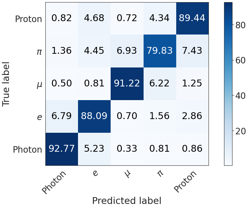
PID
def plot_confusion_matrix(cm,
                          normalize=False,
                          title=None,
                          cmap=plt.cm.Blues,
                         xlabel='Predicted label',
                         ylabel='True label'):
    """
    This function prints and plots the confusion matrix.
    Normalization can be applied by setting `normalize=True`.
    """
    #xticklabels = ['HIP', 'MIP', 'Shower', 'Delta', 'Michel']

    xticklabels = ['Photon', '$e$', '$\mu$', '$\pi$', 'Proton']
    if cm.shape[1] > 5:
        xticklabels.append('Ghost')
    #     if cm.shape[1] > 5:
    #         xticklabels.append('Ghost')

    fig, ax = plt.subplots()
    print(cm.shape)
    im = ax.imshow(cm, interpolation='nearest', cmap=cmap)
    ax.figure.colorbar(im, ax=ax)
    #labels = ['HIP', 'MIP', 'Shower', 'Delta', 'Michel']
    labels = ['Photon', '$e$', '$\mu$', '$\pi$', 'Proton']
    # We want to show all ticks...
    ax.set(xticks=np.arange(cm.shape[1]),
           yticks=np.arange(cm.shape[0]),
           # ... and label them with the respective list entries
           xticklabels=xticklabels, yticklabels=labels,
           title=title,
           ylabel=ylabel,
           xlabel=xlabel,
           ylim=(-0.5, cm.shape[0]-0.5))

    # Rotate the tick labels and set their alignment.
    plt.setp(ax.get_xticklabels(), rotation=45, ha="right",
             rotation_mode="anchor")

    # Loop over data dimensions and create text annotations.
    fmt = '.2f'
    thresh = cm.max() / 2.
    for i in range(cm.shape[0]):
        for j in range(cm.shape[1]):
            ax.text(j, i, format(cm[i, j], fmt),
                    ha="center", va="center",
                    color="white" if cm[i, j] > thresh else "black")
    fig.tight_layout()
    return ax
from numpy.linalg import norm
def confusion_matrix(kinematics, num_classes):
    x = np.zeros((num_classes, num_classes))
    for c in range(num_classes):
        for c2 in range(num_classes):
            x[c][c2] =  np.count_nonzero((kinematics['true_type'] == c) & (kinematics['pred_type'] == c2) )
        #x[c][-1] = np.nansum(metrics['num_true_pix_class%d' % c]-metrics['num_true_deghost_pix_class%d' % c])
    return x / x.sum(axis=1, keepdims=True)
kinematics = pd.read_csv(os.path.join(METRICS_FOLDER, "pid-metrics.csv"))

seaborn.set(style="white", font_scale=2.5)
plot_confusion_matrix(np.array(confusion_matrix(kinematics, 5)*100))
#plt.savefig("confusion_matrix.png", transparent=True)
seaborn.set(rc={
    'figure.figsize':(15, 10),
})
seaborn.set_context('talk')
(5, 5)
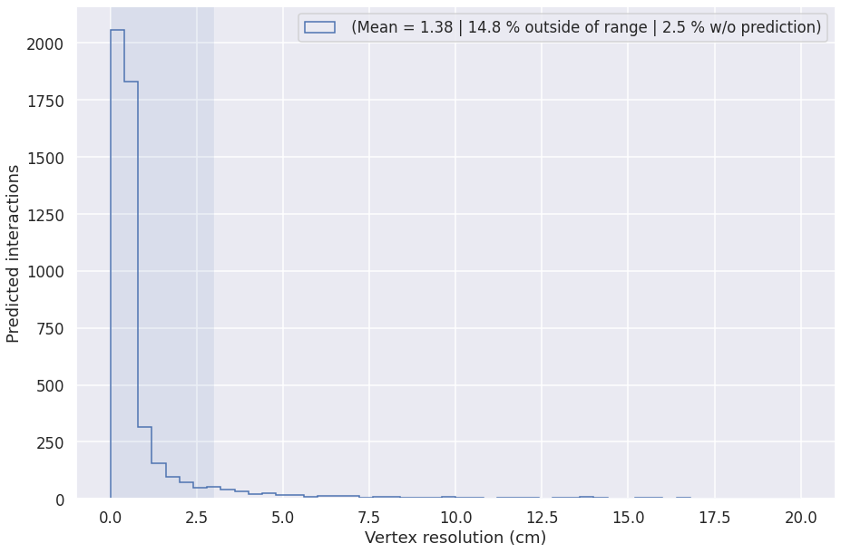
Vertex heuristic performance
This plot is computed on MPV (particle gun) interactions with at least 2 primaries.
def plot_vtx_resolution(vtx_candidates, label=''):
    vtx_predicted = (vtx_candidates['vtx_resolution'] >= 0)
    min_primaries = (vtx_candidates['num_primaries'] > 1) #& (vtx_candidates['num_pix'] > 20)
    nu_filter = (vtx_candidates['is_nu'] > 0)
    r = [0, 20]

    vtx_filter = vtx_predicted & min_primaries & nu_filter

    no_prediction = np.count_nonzero(~vtx_predicted & min_primaries & nu_filter)/np.count_nonzero(min_primaries & nu_filter) * 100
    outside = np.count_nonzero(vtx_filter & (vtx_candidates['vtx_resolution'] > r[1]))/np.count_nonzero(vtx_filter)*100
    mean_range = [0, 3]
    mean = vtx_candidates['vtx_resolution'][vtx_filter][(vtx_candidates['vtx_resolution'][vtx_filter] > mean_range[0]) & (vtx_candidates['vtx_resolution'][vtx_filter] < mean_range[1])].mean()
    plt.hist(vtx_candidates['vtx_resolution'][vtx_filter]*0.3, range=r, bins=50, histtype='step', label='%s (Mean = %.2f | %.1f %% outside of range | %.1f %% w/o prediction)' % (label, mean, outside, no_prediction))
    plt.xlabel('Vertex resolution (cm)')
    plt.ylabel('Predicted interactions')

    plt.gca().axvspan(mean_range[0], mean_range[1], alpha=0.1)
    plt.legend()
vtx_candidates = pd.read_csv(os.path.join(METRICS_FOLDER, "vertex-candidates.csv"))

plot_vtx_resolution(vtx_candidates)