Overview of the reconstruction chain
Let’s look at the big picture first before we dive into the code details of visualization and configuration.
Fig. 7 Overview of the full chain
Warning
TODO Add event displays for each stage (true label)
Input: LArTPC images
LArTPC detectors come in two flavors: wire LArTPCs (2D images, three views) and pixel LArTPCs (native 3D images).
lartpc_mlreco3d is mostly targeting 3D datasets.
An algorithm written by T. Usher, called Cluster3D, can be run on the wire LArTPC data (consisting of three
complementary 2D images) to create corresponding 3D points. This algorithm has inefficiencies - it creates
some ghost points along the way, i.e. 3D points that are mistakenly reconstructed by the algorithm but should
not exist.
In practice, the input 3D images come from a ROOT file that was created with LArCV (a C++ library to process LArTPC images). The reconstruction chain has I/O parsers that read the LArCV file and create a sparse 3D input (list of 3D coordinates for non-zero voxels) for the downstream networks.
Semantic segmentation with UResNet
Semantic segmentation is a jargon term that means pixel-wise classification. The current datasets distinguish between 5 classes (6 if the input includes ghost points):
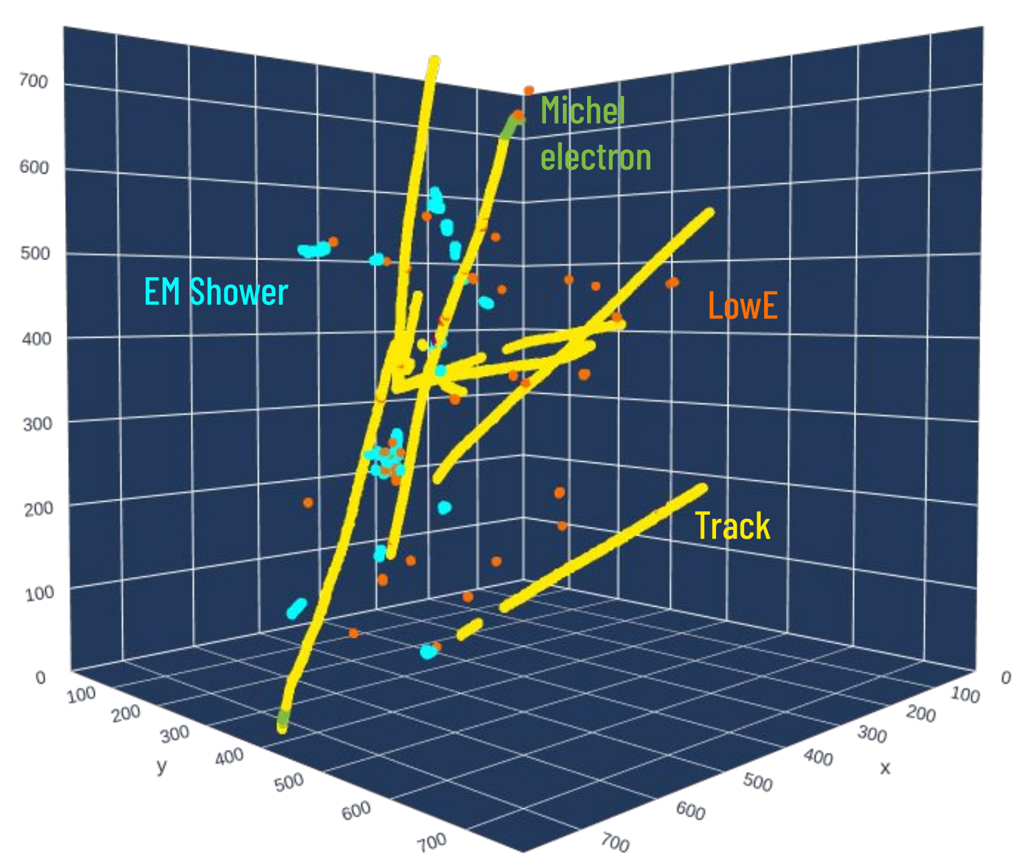
Fig. 8 Example image - only 4 semantic classes shown here.
Electromagnetic showers (e.g. electrons, photons = gammas)
Track-like particles (e.g. muons, protons, pions)
Delta rays (electrons knocked off from hard scattering)
Michel electrons (coming from muon decay)
Low energy depositions
(if enabled) Ghost points
UResNet is a network architecture widely used for semantic segmentation tasks. In our chain it predicts a 5 classes voxel-wise classification, as well as a binary (ghost / non-ghost) classification mask if ghost points are present.
Points of interest with PPN
PPN stands for Point Proposal Network. This network is made of just three layers attached to the UResNet
network at different stages. It predicts points of interest in the image:
start point of electromagnetic showers
start and end point of tracks
For each point of interest, PPN predicts several things:
3D offset coordinates from the voxel center
5 classes classification scores (same 5 classes as in the semantic segmentation above)
(experimental) for track points only, a start vs end point binary classification score
Particle clustering
The next stage is to cluster the voxels into individual particle instances. The chain clusters separately track-like particles and shower-like particles.
Shower clustering (GNN)
The chain uses a GNN (graph neural network). It first runs DBSCAN on the shower voxels to create shower fragments. For each of these fragments, we compute geometrical features that we feed to the GNN.
Track clustering (SPICE)
For track-like particles, the chain uses either SPICE or GraphSPICE (improved version of SPICE). The idea is to teach the network how to embed the voxels into a different (higher dimensional) embedding space, and to run a clustering strategy in this space.
Interaction clustering (GNN)
Now that we have individual particle instances from the previous stage, the chain will use a different GNN network to predict interactions, i.e. groups of particle instances that have interacted together. Each node in the graph is a predicted particle instance, and we are trying to predict which edges should exist between these nodes.
In addition to predicting interaction groups, this stage also predicts for each particle instance:
particle identification (PID), i.e. the type of the particle (TODO list here different types)
a binary classification primary / non-primary particle. Particles coming directly out of an interaction vertex are labelled as primary particles.
Kinematics and particle hierarchy (GNN)
Yet another GNN network predicts the particle hierarchy: interactions create parent-child relationships between particle instances, and the GNN predicts a binary on-off classification for each edge of a complete graph connecting all the particle instances (nodes).
In addition to the particle hierarchy, the GNN also predicts for each particle instance kinematics variables (momentum).
Cosmic discrimination
For each predicted interaction group, we want to know whether it is a cosmic (background) interaction or a neutrino (signal) interaction.
Hopefully, this gives you enough of a flavor of the reconstruction chain and you are ready (no, excited!) to see some visualizations of the chain input/output.